Explaining a Machine Learning Model: ICE and PD
Tutorial Contents
In this tutorial, we show how to gather some insights about inner workings of a predictive model by using Individual Conditional Expectation (ICE) and Partial Dependence (PD) tools. We highlight pros of these tools and point out a few caveats that every person using them should be aware of. Analysing ICE and PD of a predictive model allows us to understand how the model’s predictions change (on average) as we vary one of the features.
As with all the other tutorials, we first need to import all the necessary dependencies and load a data set. For this tutorial we will use the Iris data set:
>>> import numpy as np
>>> import matplotlib.pyplot as plt

>>> import fatf.utils.data.datasets as fatf_datasets
>>> iris_data_dict = fatf_datasets.load_iris()
>>> iris_data = iris_data_dict['data']
>>> iris_target = iris_data_dict['target'].astype(int)
Since this tutorial is focused on explaining a predictive model, we need to train one first:
>>> import fatf.utils.models as fatf_models
>>> clf = fatf_models.KNN()
>>> clf.fit(iris_data, iris_target)
Both ICE and PD will tell us how the probability of a selected class changes as we move along one of the features – for a selected subset of data points either individually (ICE) or on average (PD) – therefore we need to choose what class we are interested in, which feature want to inspect and what subset of data points we will use for the ICE/PD evaluation. Let us focus on the virginica iris type:
>>> iris_target_names = iris_data_dict['target_names']

>>> selected_class_name = 'virginica'
>>> selected_class_index = np.where(
...     iris_target_names == selected_class_name)
>>> selected_class_index = selected_class_index[0]
>>> selected_class_index.shape
(1,)
>>> selected_class_index = int(selected_class_index[0])
We want know how does the sepal width (cm) feature influence the model’s predictions of this class:
>>> iris_feature_names = iris_data_dict['feature_names']

>>> selected_feature_name = 'sepal width (cm)'
>>> selected_feature_index = np.where(
...     iris_feature_names == selected_feature_name)
>>> selected_feature_index = selected_feature_index[0]
>>> selected_feature_index.shape
(1,)
>>> selected_feature_index = int(selected_feature_index[0])
For ICE/PD evaluation we will use the first 10 points of each class. Since the
data points are ordered we will use [0:10] indices for the first class,
[50:60] for the second one and [100:110] for the last one:
>>> indices_data_eval = (
...     list(range(0, 10)) + list(range(50, 60)) + list(range(100, 110)))
>>> len(indices_data_eval)
30

>>> iris_data_eval = iris_data[indices_data_eval, :]
>>> iris_target_eval = iris_target[indices_data_eval]

>>> np.unique(iris_target_eval, return_counts=True)
(array([0, 1, 2]), array([10, 10, 10]))
Now, we are ready to pry this black box open.
Individual Conditional Expectation
Let us dive straight in and see how the probability of the virginica class
changes given the sepal width for the selected data points using the fatf.transparency.models.feature_influence.individual_conditional_expectation
function:
>>> import fatf.transparency.models.feature_influence as fatf_fi
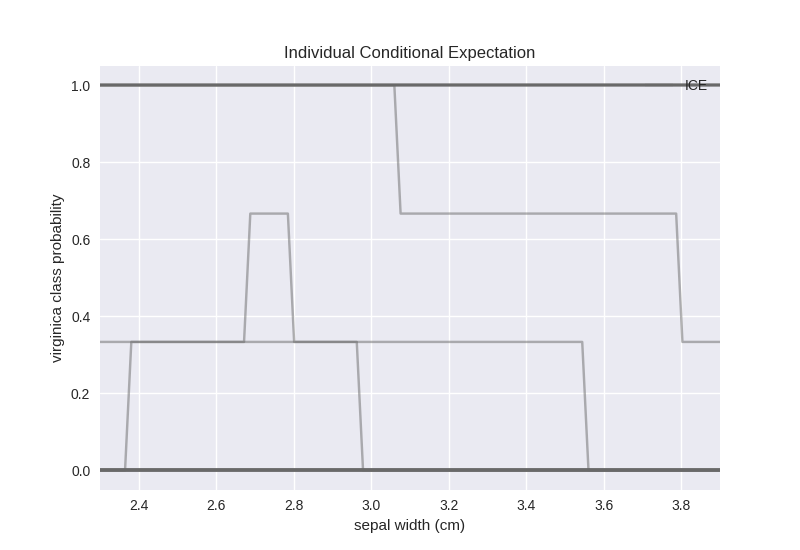
>>> ice_array, ice_linspace = fatf_fi.individual_conditional_expectation(
... iris_data_eval, clf, selected_feature_index, steps_number=100)
>>> ice_array.shape
(30, 100, 3)
To make sense of the ICE array – which holds probabilities output by the
model for 3 classes of the 30 selected data points with the selected
feature varied between its minimum and maximum over a 100 uniform steps –
we can visualise it with a plotting function built into FAT Forensics:
>>> import fatf.vis.feature_influence as fatf_vis_fi

>>> ice_plot = fatf_vis_fi.plot_individual_conditional_expectation(
...    ice_array,
...    ice_linspace,
...    selected_class_index,
...    class_name=selected_class_name,
...    feature_name=selected_feature_name)
Note
Blockiness of the ICE Plot
The ICE plot may seem blocky. This effect is due to the model being a k-Nearest Neighbour classifier (by default k is equal to 3) with the probability that it outputs being the proportion of the neighbours of a given class. Therefore, 4 different probability levels can be observed:
0 – none of the neighbours is of virginica class,
0.33 – one of the neighbours is of virginica class,
0.66 – two of the neighbours are of virginica class, and
1 – all of the neighbours are of virginica class.
The plot shows that for some of the data points the sepal width feature does not have any effect on the prediction – 0 and 1 probabilities of the virginica class – whereas for others it matters. This is not very informative. Let us separate these lines based on the ground truth (target vector) and inspect the results:
>>> iris_target_names[0]
'setosa'
>>> ice_plot_0 = fatf_vis_fi.plot_individual_conditional_expectation(
...    ice_array[0:10, :, :],
...    ice_linspace,
...    selected_class_index,
...    class_name=selected_class_name,
...    feature_name=selected_feature_name)
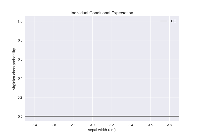
Therefore, the probability of virginica is 0 for all of our setosa examples regardless of how we modify the sepal width feature value. One conclusion that we can reach from this experiment is that this feature is not important for predicting the virginica class.
Now, let us try the versicolor examples:
>>> iris_target_names[1]
'versicolor'
>>> ice_plot_1 = fatf_vis_fi.plot_individual_conditional_expectation(
...    ice_array[10:20, :, :],
...    ice_linspace,
...    selected_class_index,
...    class_name=selected_class_name,
...    feature_name=selected_feature_name)
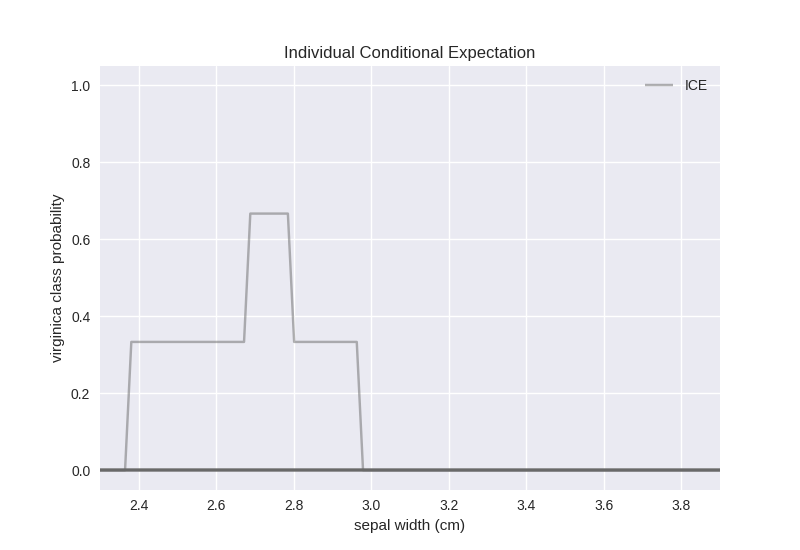
Our versicolor examples indicate some dependence on the sepal width feature value in the region between 2.4 and 3. Given that there is just one example and that it would only be classified as virginica for sepal width between 2.7 and 2.8 there is nothing definitive that we can say about this dependence. One observation worth mentioning is that there has to be some sort of feature correlation/dependence in the data set that result in this behaviour for the single data point.
Finally, let us see how the probability of virginica changes based on the sepal width feature for the actual examples of virginica class:
>>> iris_target_names[2]
'virginica'
>>> ice_plot_2 = fatf_vis_fi.plot_individual_conditional_expectation(
...    ice_array[20:30, :, :],
...    ice_linspace,
...    selected_class_index,
...    class_name=selected_class_name,
...    feature_name=selected_feature_name)
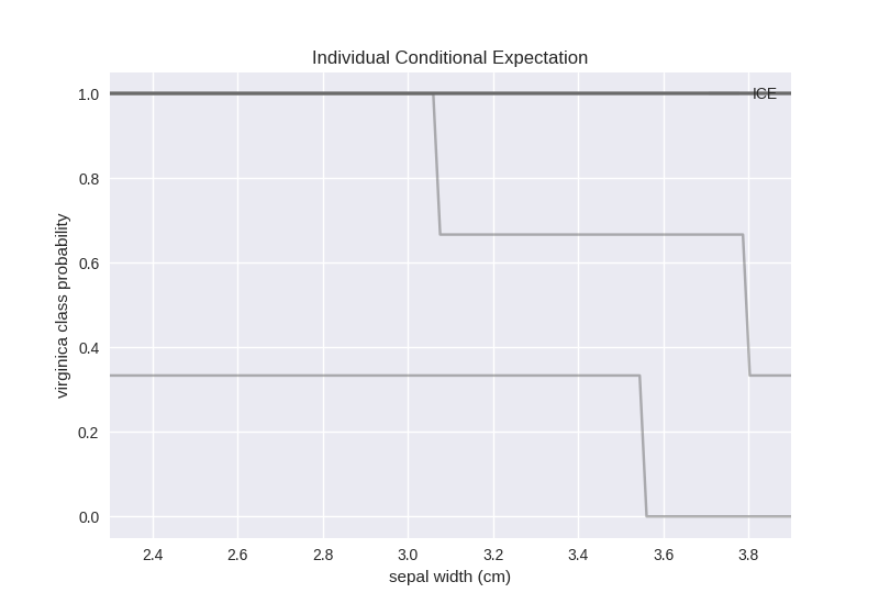
Other than the two visible points, the model predicts probability of 1 for all the other ones. However, one of this “unstable” data points – the lowest line – is misclassified by the model regardless of the value of the sepal width feature, whereas the other data point would only be misclassified for a sepal width larger than 3.8.
Given all these experiments we can conclude that telling apart the virginica class from the other two is not straight forward using the sepal width feature. For completeness, let us pick another feature, which we know (from experience) is a good predictor for the virginica class – petal length:
>>> other_feature_index = 2
>>> other_feature_name = iris_feature_names[other_feature_index]
>>> other_feature_name
'petal length (cm)'

>>> n_ice_arr, n_ice_lin = fatf_fi.individual_conditional_expectation(
...     iris_data_eval, clf, other_feature_index, steps_number=100)

>>> n_ice_plot = fatf_vis_fi.plot_individual_conditional_expectation(
...    n_ice_arr,
...    n_ice_lin,
...    selected_class_index,
...    class_name=selected_class_name,
...    feature_name=other_feature_name)
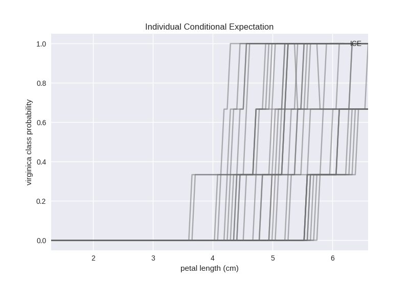
Petal length is clearly a good predictor for the virginica class as for values of this feature falling below 3.6 there is 0 probability for our examples to be of virginica type, but above that the probability of this class grows rapidly.
Note
Grouping Based on the Ground Truth
In this example we were able to separate data points into three bins based on their ground truth value since we know the ordering of the data in the array. For more complex cases you may want to use the grouping funcitonctionality implemented in the FAT Forensics package. Please consult the Exploring the Grouping Concept – Defining Sub-Populations tutorial for more information.
Evaluation Data Density
In the example above we only used 30 data points, which is not enough to make any meaningful conclusions. For the virginica data points we have noticed that sepal width above 3.8 causes one of the data points to be misclassified, but should we trust this observation? That depends on how many data points we have seen in this region. For some values of this feature we may have not observed any real data points, which means that the model is likely to output predictions that are not meaningful in this region. However, when evaluating the ICE of a model we plot these predictions anyway. Therefore, we should be careful when reading these plots and inspect distribution of the feature that we inspect to validate the effect presented in an ICE plot.
Given this observation, let us see the distribution of the sepal width feature for the full Iris data set:
>>> hist_plot = plt.figure()
>>> hist = plt.hist(iris_data[:, selected_feature_index], bins=30)
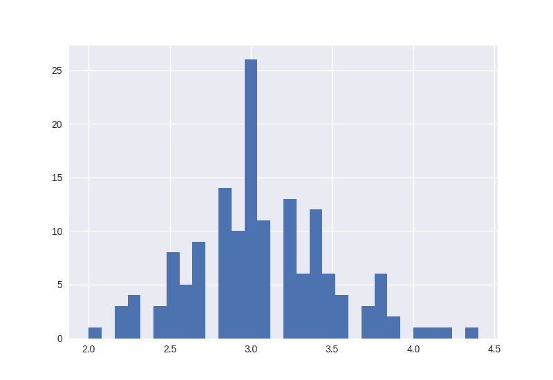
We can clearly see that there are only a few (training) data points that have the sepal width feature above 3.8. Therefore, before we draw a conclusion that sepal width above 3.8 indicates that it is not a virginica iris, we should first make additional experiments.
Partial Dependence
A complement of the ICE is Partial Dependence that aims at finding average,
rather than individual, feature influence on a selected class. To get a PD
array we could use the fatf.transparency.models.feature_influence.partial_dependence function, however this would mean recomputing the ICE
array. To avoid this expensive computation, we will use the fatf.transparency.models.feature_influence.partial_dependence_ice function that
can reuse an already existing ICE array:
>>> pd_array = fatf_fi.partial_dependence_ice(ice_array)
which we can plot with:
>>> pd_plot = fatf_vis_fi.plot_partial_dependence(
...     pd_array,
...     ice_linspace,
...     selected_class_index,
...     class_name=selected_class_name,
...     feature_name=selected_feature_name)
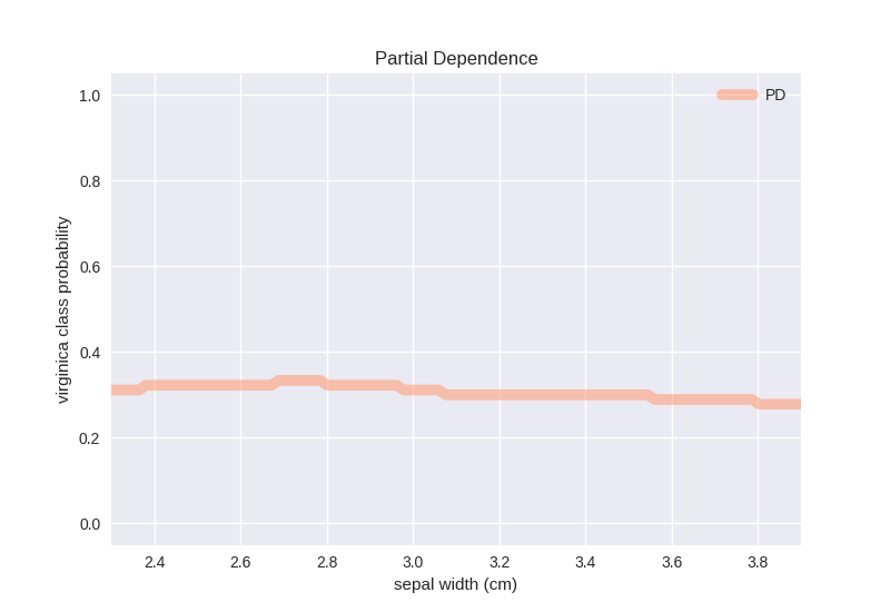
The PD plot, surprisingly, indicates that the sepal width feature does not influence the probability of the virginica class (on average) and regardless of the value that this feature takes the probability of virginica is around 0.35.
Misleading Average
The surprising result sown above is the effect of PD taking an average over all the individual effects (ICE). This can often be misleading. To avoid misinterpreting PD results, we often overlay it on top of an ICE plot:
>>> ice_re_plot = fatf_vis_fi.plot_individual_conditional_expectation(
...     ice_array,
...     ice_linspace,
...     selected_class_index,
...     class_name=selected_class_name,
...     feature_name=selected_feature_name)
>>> ice_re_plot_figure, ice_re_plot_axis = ice_re_plot
>>> pd_re_plot = fatf_vis_fi.plot_partial_dependence(
...     pd_array,
...     ice_linspace,
...     selected_class_index,
...     class_name=selected_class_name,
...     feature_name=selected_feature_name,
...     plot_axis=ice_re_plot_axis)
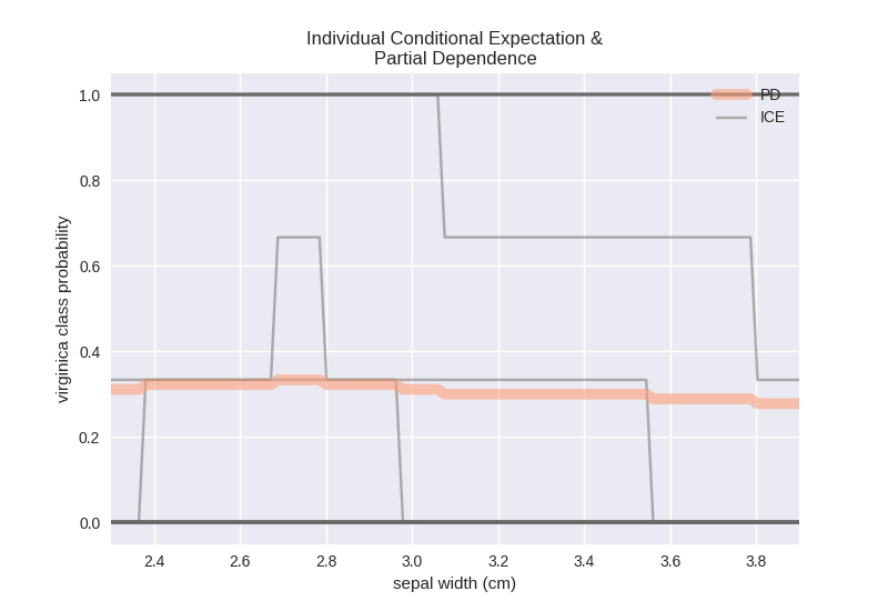
Such plot presents a full picture and allows us to draw conclusions about the usefulness of the PD curve.
This tutorial walked through using Individual Conditional Expectation and Partial Dependence to explain influence of features on predictions of a model. We saw how to use both these functions and what to look for when interpreting their results.
In the next tutorial we will see how to assess transparency of predictions with counterfactuals and LIME. If you are looking for a tutorial on explaining data sets, please have a look at the Using Grouping to Inspect a Data Set – Data Transparency section of the Exploring the Grouping Concept – Defining Sub-Populations tutorial.
Relevant FAT Forensics Examples
The following examples provide more structured and code-focused use-cases of the ICE and PD functionality:

