How to build LIME yourself (bLIMEy) – Surrogate Tabular Explainers

How-to Guide Contents

This how-to guide illustrates how to construct a local surrogate model on top of a black-box model and use it to generate explanations of selected predictions of the black-box model.

This how-to guide requires scikit-learn package as it uses ridge regression and decision tree predictors (implemented therein) as local surrogate models.

Each surrogate explainer is composed of three main parts:

• interpretable data representation;

• data sampling; and

• explanation generation.

Choosing a particular algorithm for each of these components shapes the type of surrogate explanations that can be generated with the final explainer. (The theoretical considerations for each component can be found in Surrogate Transparency User Guide, [SOKOL2019BLIMEY] and the Jupyter Notebook distributed with the latter manuscript.) In this how-to guide we will show how to build the tabular LIME explainer [RIBEIRO2016WHY] (with fixed sampling procedure [SOKOL2019BLIMEY] and the sampling algorithm replaced with MixuP – fatf.utils.data.augmentation.Mixup) and a simple tree-based surrogate.

Two similar surrogate explainer are already distributed with this package: fatf.transparency.predictions.surrogate_explainers.TabularBlimeyLime and fatf.transparency.predictions.surrogate_explainers.TabularBlimeyTree. However, the LIME explainer implementation is the exact replica of its official implementation, hence it does the “reverse sampling”, which introduces randomness to the explainer. Both of these classes provide usage convenience – no need to build the explainers from scratch – in exchange for lack of flexibility – none of the three aforementioned components can be customised.

Note

Deploying Surrogate Explainers

You may want to consider using the abstract fatf.transparency.predictions.surrogate_explainers.SurrogateTabularExplainer class to implement a custom surrogate explainer for tabular data. This abstract class implements a series of input validation steps and internal attribute computation that make implementing a custom surrogate considerably easier.

SOKOL2019BLIMEY(1,2)

Sokol, K., Hepburn, A., Santos-Rodriguez, R. and Flach, P., 2019. bLIMEy: Surrogate Prediction Explanations Beyond LIME. 2019 Workshop on Human-Centric Machine Learning (HCML 2019). 33rd Conference on Neural Information Processing Systems (NeurIPS 2019), Vancouver, Canada. arXiv preprint arXiv:1910.13016. URL https://arxiv.org/abs/1910.13016.

RIBEIRO2016WHY

Ribeiro, M.T., Singh, S. and Guestrin, C., 2016, August. Why should I trust you?: Explaining the predictions of any classifier. In Proceedings of the 22nd ACM SIGKDD international conference on knowledge discovery and data mining (pp. 1135-1144). ACM.

Setup

First, let us set the random seed to ensure reproducibility of the results:

>>> import fatf

>>> fatf.setup_random_seed(42)

We will also need numpy:

>>> import numpy as np

Next, we need to load the IRIS data set, which we will use for this how-to guide:

>>> import fatf.utils.data.datasets as fatf_datasets

>>> iris_data_dict = fatf_datasets.load_iris()
>>> iris_data = iris_data_dict['data']
>>> iris_target = iris_data_dict['target']
>>> iris_feature_names = iris_data_dict['feature_names'].tolist()
>>> iris_target_names = iris_data_dict['target_names'].tolist()

Now, we will train a black-box model – k-nearest neighbours predictor:

>>> import fatf.utils.models.models as fatf_models

>>> blackbox_model = fatf_models.KNN(k=3)
>>> blackbox_model.fit(iris_data, iris_target)

and compute its training set accuracy:

>>> import sklearn.metrics

>>> predictions = blackbox_model.predict(iris_data)
>>> sklearn.metrics.accuracy_score(iris_target, predictions)
0.96

As you can see, the IRIS dataset is reasonably easy for the k-NN classifier and it achieves a high accuracy. Next, we need to choose a data point for which we will generate an explanation with respect to this model:

>>> data_point = iris_data[0]
>>> data_point
array([5.1, 3.5, 1.4, 0.2], dtype=float32)

>>> data_point_probabilities = blackbox_model.predict_proba(
...     data_point.reshape(1, -1))[0]
>>> data_point_probabilities
array([1., 0., 0.])
>>> data_point_prediction = data_point_probabilities.argmax(axis=0)
>>> data_point_prediction
0
>>> data_point_class = iris_target_names[data_point_prediction]
>>> data_point_class
'setosa'

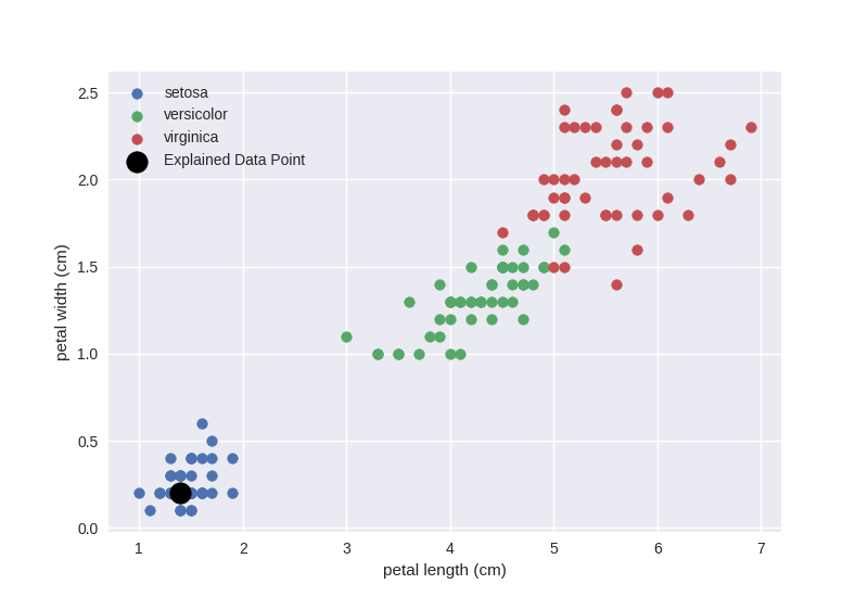
Let us visualise where the data_point lies in the data set by plotting the last two dimensions of the data and highlighting the data_point:

>>> import matplotlib.pyplot as plt

>>> iris_feature_names[2:]
['petal length (cm)', 'petal width (cm)']

>>> _ = plt.figure()
>>> _ = plt.scatter(
...     iris_data[1:50, 2],
...     iris_data[1:50, 3],
...     label=iris_target_names[0])
>>> _ = plt.scatter(
...     iris_data[50:100, 2],
...     iris_data[50:100, 3],
...     label=iris_target_names[1])
>>> _ = plt.scatter(
...     iris_data[100:150, 2],
...     iris_data[100:150, 3],
...     label=iris_target_names[2])
>>> _ = plt.scatter(
...     data_point[2],
...     data_point[3],
...     label='Explained Data Point',
...     s=200, c='k')

>>> _ = plt.xlabel(iris_feature_names[2])
>>> _ = plt.ylabel(iris_feature_names[3])
>>> _ = plt.legend()

Surrogate Linear Model (LIME)

We will use the quartile discretisation for the interpretable data representation:

>>> import fatf.utils.data.discretisation as fatf_discretisation

>>> discretiser = fatf_discretisation.QuartileDiscretiser(
...     iris_data,
...     feature_names=iris_feature_names)

Mixup for data sampling:

>>> import fatf.utils.data.augmentation as fatf_augmentation

>>> augmenter = fatf_augmentation.Mixup(iris_data, ground_truth=iris_target)

and a ridge regression for explanation generation:

>>> import sklearn.linear_model

>>> lime = sklearn.linear_model.Ridge()

Data Augmentation

First, we will sample new data in the neighbourhood of the selected data_point, predict them with the black-box model and plot them:

>>> sampled_data = augmenter.sample(data_point, samples_number=50)
>>> sampled_data_probabilities = blackbox_model.predict_proba(sampled_data)

>>> sampled_data_predictions = sampled_data_probabilities.argmax(axis=1)
>>> sampled_data_0_indices = np.where(sampled_data_predictions == 0)[0]
>>> sampled_data_1_indices = np.where(sampled_data_predictions == 1)[0]
>>> sampled_data_2_indices = np.where(sampled_data_predictions == 2)[0]

>>> _ = plt.figure()
>>> _ = plt.scatter(
...     iris_data[1:50, 2],
...     iris_data[1:50, 3],
...     label=iris_target_names[0])
>>> _ = plt.scatter(
...     iris_data[50:100, 2],
...     iris_data[50:100, 3],
...     label=iris_target_names[1])
>>> _ = plt.scatter(
...     iris_data[100:150, 2],
...     iris_data[100:150, 3],
...     label=iris_target_names[2])
>>> _ = plt.scatter(
...     data_point[2],
...     data_point[3],
...     label='Explained Data Point: {}'.format(data_point_class),
...     s=200,
...     c='k')

>>> _ = plt.scatter(
...     sampled_data[sampled_data_0_indices, 2],
...     sampled_data[sampled_data_0_indices, 3],
...     label='Augmented Data: {}'.format(iris_target_names[0]))
>>> _ = plt.scatter(
...     sampled_data[sampled_data_1_indices, 2],
...     sampled_data[sampled_data_1_indices, 3],
...     label='Augmented Data: {}'.format(iris_target_names[1]))
>>> _ = plt.scatter(
...     sampled_data[sampled_data_2_indices, 2],
...     sampled_data[sampled_data_2_indices, 3],
...     label='Augmented Data: {}'.format(iris_target_names[2]))

>>> _ = plt.xlabel(iris_feature_names[2])
>>> _ = plt.ylabel(iris_feature_names[3])
>>> _ = plt.legend()

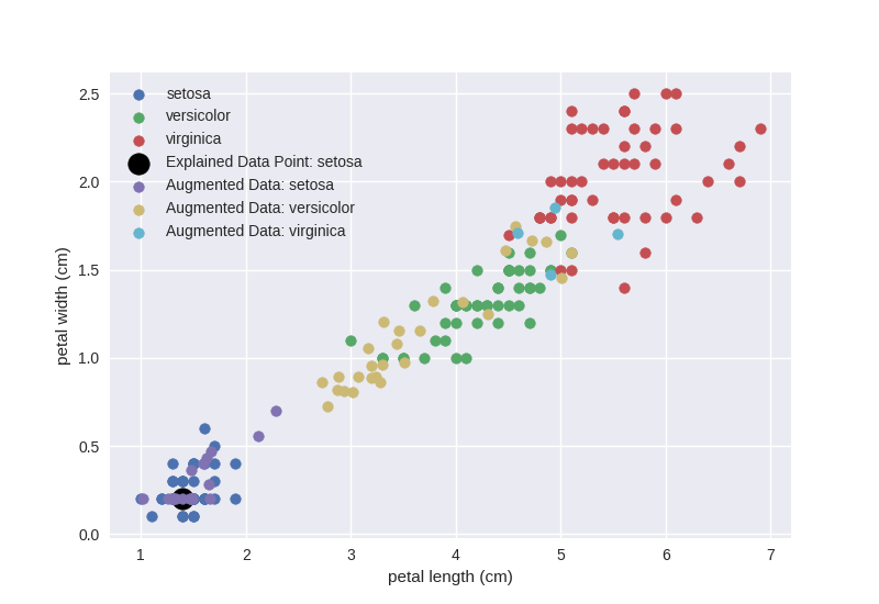
In case of LIME we use the probabilistic output of the black-box classifier as the local model – ridge regression – is fitted against the probabilities of a selected class. When using any other model (cf. the decision tree surrogate section below) it is possible to use class predictions instead. Using the probabilistic output of the black-box model also entails training the local model as one-vs-rest for a selected class to be explained. In this case we will explain the class to which the selected data_point belongs: 'setosa'.

Interpretable Representation

LIME introduces an explicit interpretable representation – discretisation of continuous features – to improve comprehensibility of explanations. This step may not be necessary for other choices of local surrogates (cf. the decision tree surrogate section below) but for LIME it allows the explanation to indicate how moving the data point out of each of the discretised bins would affect the prediction. The exact steps taken by LIME are described in the documentation of the fatf.transparency.predictions.surrogate_explainers.TabularBlimeyLime class.

First, we transform the selected data_point and the data sampled around it into the interpretable representation, i.e., we discretise them:

>>> data_point_discretised = discretiser.discretise(data_point)
>>> sampled_data_discretised = discretiser.discretise(sampled_data)

Next, we create a new representation of the discretised data, which indicates whether for each discretised feature of the sampled data whether it is the same as the bin to which the data_point belongs or not:

>>> import fatf.utils.data.transformation as fatf_transformation

>>> sampled_data_binarised = fatf_transformation.dataset_row_masking(
...     sampled_data_discretised, data_point_discretised)

Let us show how this affects the first sampled data point:

>>> data_point_discretised
array([0, 3, 0, 0], dtype=int8)
>>> sampled_data_discretised[0, :]
array([1, 3, 0, 0], dtype=int8)
>>> sampled_data_binarised[0, :]
array([0, 1, 1, 1], dtype=int8)

Explanation Generation

Finally, we train a local linear (ridge) regression to the locally sampled, discretised and binarised data and extract the explanation from its coefficient. To enforce the locality of the explanation even further, we first calculate the distances between the binarised data_point and the sampled data and kernelise these distances (with an exponential kernel) to get data point weights. We use the \(0.75 * \sqrt{\text{features number}}\) as the kernel width:

>>> import fatf.utils.distances as fatf_distances
>>> import fatf.utils.kernels as fatf_kernels

>>> features_number = sampled_data_binarised.shape[1]
>>> kernel_width = np.sqrt(features_number) * 0.75

>>> distances = fatf_distances.euclidean_point_distance(
...     np.ones(features_number), sampled_data_binarised)
>>> weights = fatf_kernels.exponential_kernel(
...     distances, width=kernel_width)

We use np.ones(...) here as it is equivalent to binarising the data_point against itself:

>>> fatf_transformation.dataset_row_masking(
...     data_point_discretised.reshape(1, -1), data_point_discretised)
array([[1, 1, 1, 1]], dtype=int8)

As mentioned before, we will explain the 'setosa' class, which has index 0:

>>> iris_target_names.index('setosa')
0

Therefore, we extract the probabilities of the first column (with index 0) from the black-box predictions:

>>> sampled_data_predictions_setosa = sampled_data_probabilities[:, 0]

Next, we do weighted feature selection to introduce sparsity to the explanation. To this end, we use k-LASSO and select 2 features with it:

>>> import fatf.utils.data.feature_selection.sklearn as fatf_feature_ssk

>>> lasso_indices = fatf_feature_ssk.lasso_path(
...     sampled_data_binarised, sampled_data_predictions_setosa, weights, 2)

Now, we prepare the binarised data set for training the surrogate ridge regression by extracting the features chosen with lasso:

>>> sampled_data_binarised_2f = sampled_data_binarised[:, lasso_indices]

and retrieve the names of these two binary features (in the interpretable representation):

>>> interpretable_feature_names = []
>>> for feature_index in lasso_indices:
...     bin_id = data_point_discretised[feature_index].astype(int)
...     interpretable_feature_name = (
...         discretiser.feature_value_names[feature_index][bin_id])
...     interpretable_feature_names.append(interpretable_feature_name)
>>> interpretable_feature_names
['*petal length (cm)* <= 1.60', '*petal width (cm)* <= 0.30']

Last but not least, we train a local weighted ridge regression:

>>> lime.fit(
...     sampled_data_binarised_2f,
...     sampled_data_predictions_setosa,
...     sample_weight=weights)
Ridge()

and explain the data_point with its coefficients:

>>> for name, importance in zip(interpretable_feature_names, lime.coef_):
...     print('->{}<-: {}'.format(name, importance))
->*petal length (cm)* <= 1.60<-: 0.4297609038698995
->*petal width (cm)* <= 0.30<-: 0.37901863586706086

This explanation agrees with our intuition as based on the data scatter plot if the petal length (x-axis) is larger than 1.6, we are moving outside of the blue cluster (setosa) and if petal width (y-axis) is larger than 0.3, we are also moving outside of the blue cluster.

---

We leave explaining the other classes as an exercise for the reader.

Surrogate Tree

A linear regression fitted as one-vs-rest to probabilities of a selected class is not the only surrogate that can give us some insights into the black-box model operations. Next, we train a shallow local decision tree.

Since a decision tree can learn its own interpretable representation – the feature splits – we can use the sampled data in its original domain to train the surrogate tree. Furthermore, by limiting the depth of the tree we force it to do feature selection, hence no need for an auxiliary dimensionality reduction. To this end, we just need to compute weights between the sampled data and the data_point in this domain:

>>> features_number = sampled_data.shape[1]
>>> kernel_width = np.sqrt(features_number) * 0.75

>>> distances = fatf_distances.euclidean_point_distance(
...     data_point, sampled_data)
>>> weights = fatf_kernels.exponential_kernel(
...     distances, width=kernel_width)

Lastly, we need to decide whether we want to train the tree as a regressor for probabilities of one of the classes (as with LIME) or use a classification tree. We will go with the latter option. Now, we have a choice between training the tree as a multi-class classifier for all of the classes or as one-vs-rest for a selected class. The advantage of the former is that the same tree can be used to explain all of the classes at once, therefore we will go with a multi-class classification tree:

>>> import sklearn.tree

>>> blimey_tree = sklearn.tree.DecisionTreeClassifier(max_depth=3)
>>> blimey_tree.fit(
...     sampled_data, sampled_data_predictions, sample_weight=weights)
DecisionTreeClassifier(max_depth=3)

One possible explanation that we can extract from the tree is feature importance:

>>> for n_i in zip(iris_feature_names, blimey_tree.feature_importances_):
...     name, importance = n_i
...     print('->{}<-: {}'.format(name, importance))
->sepal length (cm)<-: 0.0
->sepal width (cm)<-: 0.0057061683826981156
->petal length (cm)<-: 0.008758435540648965
->petal width (cm)<-: 0.9855353960766529

This explanation agrees with LIME but is not as informative as the one derived with LIME. A better explanation is the tree structure itself:

>>> blimey_tree_text = sklearn.tree.export_text(
...     blimey_tree, feature_names=iris_feature_names)
>>> print(blimey_tree_text)
|--- petal width (cm) <= 0.71
|   |--- class: 0
|--- petal width (cm) >  0.71
|   |--- petal length (cm) <= 4.58
|   |   |--- class: 1
|   |--- petal length (cm) >  4.58
|   |   |--- sepal width (cm) <= 2.91
|   |   |   |--- class: 2
|   |   |--- sepal width (cm) >  2.91
|   |   |   |--- class: 1

Let us recall the sampled data:

>>> _ = plt.figure()
>>> _ = plt.scatter(
...     sampled_data[sampled_data_0_indices, 2],
...     sampled_data[sampled_data_0_indices, 3],
...     label='Augmented Data: {}'.format(iris_target_names[0]))
>>> _ = plt.scatter(
...     sampled_data[sampled_data_1_indices, 2],
...     sampled_data[sampled_data_1_indices, 3],
...     label='Augmented Data: {}'.format(iris_target_names[1]))
>>> _ = plt.scatter(
...     sampled_data[sampled_data_2_indices, 2],
...     sampled_data[sampled_data_2_indices, 3],
...     label='Augmented Data: {}'.format(iris_target_names[2]))
>>> _ = plt.scatter(
...     data_point[2],
...     data_point[3],
...     label='Explained Data Point: {}'.format(data_point_class),
...     s=200,
...     c='k')

>>> _ = plt.xlabel(iris_feature_names[2])
>>> _ = plt.ylabel(iris_feature_names[3])
>>> _ = plt.legend()

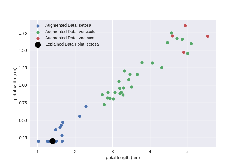
Clearly, the first split petal width (cm) <= 0.71, which is on the y-axis is enough to separate the blue cloud (setosa) from the other two classes and the petal length (cm) <= 4.58 split for petal width > 0.71 is the best we can do to separate the orange and green clouds. Had we sampled more data, the local surrogate would have better approximated the local decision boundary of the black-box model. We leave further experiments in this direction to the reader.