Measuring Robustness of a Prediction – Data Density

This example illustrates how to use a data density estimation to “measure” to what extent a prediction should be trusted.

# Author: Kacper Sokol <k.sokol@bristol.ac.uk>
# License: new BSD

import matplotlib.pyplot as plt
import numpy as np

import fatf.utils.data.datasets as fatf_datasets
import fatf.utils.models as fatf_models

import fatf.utils.data.density as fatf_density

print(__doc__)

# Prepare a colourmap
cmap = np.array([
    plt.get_cmap('Pastel1').colors[0],
    plt.get_cmap('Pastel1').colors[1],
    plt.get_cmap('Pastel1').colors[2]
])

# Load data
iris_data_dict = fatf_datasets.load_iris()
iris_X = iris_data_dict['data']
iris_y = iris_data_dict['target'].astype(int)
iris_feature_names = iris_data_dict['feature_names']
iris_class_names = iris_data_dict['target_names']

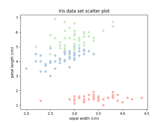
First, we visualise the data set based on two (arbitrarily chosen) features to help us guide choosing a data point in a sparse region and another one in a dense region.

# Choose 2 features
chosen_features_index = [1, 2]
chosen_features_name = iris_feature_names[chosen_features_index]

# Get a subset of the data set with these two features
iris_X_chosen_features = iris_X[:, chosen_features_index]

# Plot the dataset using the 2 selected features
plt.scatter(
    iris_X_chosen_features[:, 0], iris_X_chosen_features[:, 1], c=cmap[iris_y])
plt.title('Iris data set scatter plot')
plt.xlabel(chosen_features_name[0])
plt.ylabel(chosen_features_name[1])
plt.show()

Now, we train a predictive model on the whole data set using these two features. We will use it to evaluate the quality and robustness of the predictions it provides.

# Train a model
clf = fatf_models.KNN()
clf.fit(iris_X_chosen_features, iris_y)

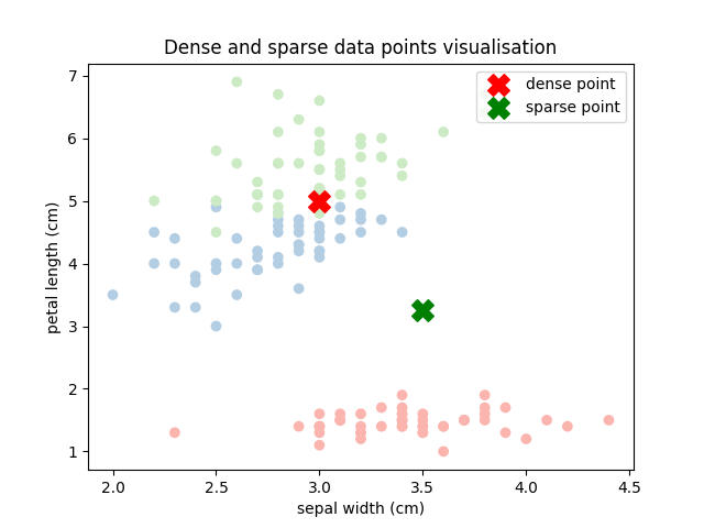
# Create two data points: one in a dense region and one in a sparse region
point_dense = np.array([[3.0, 5.0]])
point_sparse = np.array([[3.5, 3.25]])

# Plot the dense and sparse data points
plt.scatter(
    iris_X_chosen_features[:, 0], iris_X_chosen_features[:, 1], c=cmap[iris_y])
plt.scatter(
    point_dense[:, 0],
    point_dense[:, 1],
    c='r',
    s=200,
    marker='X',
    label='dense point')
plt.scatter(
    point_sparse[:, 0],
    point_sparse[:, 1],
    c='g',
    s=200,
    marker='X',
    label='sparse point')
plt.title('Dense and sparse data points visualisation')
plt.xlabel(chosen_features_name[0])
plt.ylabel(chosen_features_name[1])
plt.legend(loc='upper right')
plt.show()

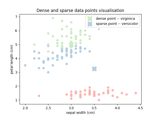
Now, let us get the predictions for both these data points.

# Predict the two data points
point_dense_prediction = clf.predict(point_dense)[0]
point_sparse_prediction = clf.predict(point_sparse)[0]

# Print out the predictions...
print('The **dense** data point is of class: {} ({}).'.format(
    iris_class_names[point_dense_prediction], point_dense_prediction))
print('The **sparse** data point is of class: {} ({}).'.format(
    iris_class_names[point_sparse_prediction], point_sparse_prediction))

# ...and plot them with the class assignment
plt.scatter(
    iris_X_chosen_features[:, 0], iris_X_chosen_features[:, 1], c=cmap[iris_y])
plt.scatter(
    point_dense[:, 0],
    point_dense[:, 1],
    c=cmap[[int(point_dense_prediction)]],
    s=200,
    marker='X',
    label='dense point -- {}'.format(iris_class_names[point_dense_prediction]))
plt.scatter(
    point_sparse[:, 0],
    point_sparse[:, 1],
    c=cmap[[int(point_sparse_prediction)]],
    s=200,
    marker='X',
    label='sparse point -- {}'.format(
        iris_class_names[point_sparse_prediction]))
plt.title('Dense and sparse data points visualisation')
plt.xlabel(chosen_features_name[0])
plt.ylabel(chosen_features_name[1])
plt.legend(loc='upper right')
plt.show()

Out:

The **dense** data point is of class: virginica (2).
The **sparse** data point is of class: versicolor (1).

Now that we know how these two data points are distributed and what class is assigned to them by the classifier we can see how a Data Density score can help us.

# Print the class names for the probability vector
print('(The probability vector is based on the following class ordering: '
      '{}.)\n'.format(iris_class_names))

# Initialise a density estimator
iris_density = fatf_density.DensityCheck(iris_X_chosen_features)

# Get a denisty estimation for the dense point
density_score_dense = iris_density.score_data_point(point_dense[0, :])
# Get the probability predictions for the dense point
probabilities_dense = clf.predict_proba(point_dense)[0]

# Get a denisty estimation for the sparse point
density_score_sparse = iris_density.score_data_point(point_sparse[0, :])
# Get the probability predictions for the sparse point
probabilities_sparse = clf.predict_proba(point_sparse)[0]

print('The prediction probabilities for the sparse data point are: {}, with a '
      'density score of {}.'.format(probabilities_sparse,
                                    density_score_sparse))

Out:

(The probability vector is based on the following class ordering: ['setosa' 'versicolor' 'virginica'].)

The prediction probabilities for the sparse data point are: [0. 1. 0.], with a density score of 0.9481604611988929.

The above result clearly shows that despite the high probability – 1 – of the versicolor class for the sparse data point, the prediction should not be trusted. The high density score for that point – 0.95 – indicates that this data point lies in a region of low density, therefore the classifier has not seen many data points in this region, hence the model is simply overconfident.

print('The prediction probabilities for the dense data point are: {}, with a '
      'density score of {}.'.format(probabilities_dense, density_score_dense))

Out:

The prediction probabilities for the dense data point are: [0.         0.33333333 0.66666667], with a density score of 0.10186747546117353.

On the other hand, the results for the dense data point, which the classifier indicates to be of class virginica with 0.67 probability, should be trusted given a low density score of 0.1. This data point clearly lies in a dense region, therefore the classifier has seen plenty of other data points in that region during the trainig procedure.